Correlation Clustering

Purpose: Show an example of how to cluster numerical features using their correlation.

The number \(\rho(X, Y) ^2\) is called the coefficient of determination. It measures how much of the variation in \(Y\) can be explained by a linear relationship to \(X\), see [1]. And \(1 - \rho(X, Y) ^2\) is the amount of unexplained variation from a linear relationship with \(X\).

References

[1] Page 212-214. Peter Olofsson. Probability, Statistics, and Stochastic Processes.

import numpy as np
import pandas as pd
import matplotlib.pyplot as plt
import matplotlib
from scipy.cluster import hierarchy as hc

matplotlib.rcParams['figure.figsize'] = (12, 12)

aarhus_apartments = pd.read_csv('aarhus_apartments.csv')

aarhus_apartments.corr()

	zip_code	price	rooms	size	build_year	latitude	longitude
zip_code	1.000000	-0.145322	-0.129532	-0.146553	0.010671	0.622659	0.244359
price	-0.145322	1.000000	0.416454	0.567506	-0.075140	0.004019	0.181975
rooms	-0.129532	0.416454	1.000000	0.795884	-0.127959	-0.050889	0.081551
size	-0.146553	0.567506	0.795884	1.000000	-0.064468	0.003794	0.225137
build_year	0.010671	-0.075140	-0.127959	-0.064468	1.000000	0.061176	0.062275
latitude	0.622659	0.004019	-0.050889	0.003794	0.061176	1.000000	0.534906
longitude	0.244359	0.181975	0.081551	0.225137	0.062275	0.534906	1.000000

def correlation_matrix(df):
    """Plots the correlation matrix.
    
    Args:
        df (pd.DataFrame): A pandas DataFrame.
    """
    corr = df.corr()
    f = plt.figure()
    plt.matshow(corr, fignum=f.number)
    plt.xticks(
        range(len(corr.columns)),
        corr.columns,
        fontsize=14,
        rotation=45,
    )
    plt.yticks(
        range(len(corr.columns)),
        corr.columns,
        fontsize=14,
    )
    cb = plt.colorbar()
    cb.ax.tick_params(labelsize=14)
    plt.title('Correlation Matrix', fontsize=16)
    plt.show()
    
correlation_matrix(aarhus_apartments)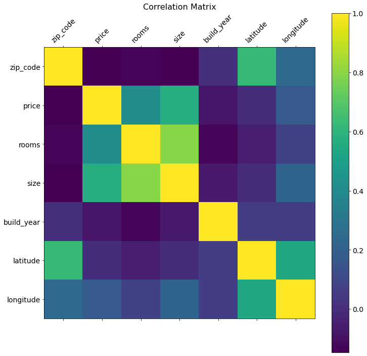

def correlation_dendogram(df, method='single'):
    """Used to plot the dendogram from a correlation matrix.
    
    1 - corr ** 2 can be interpreted as the unexplained variance
    from a linear model between a bivariate distribution (X, Y).
    This can be interpreted as a distance matrix
    
    Args:
        df (pd.DataFrame):
    """
    plt.figure()
    corr = df.corr()
    corr = np.round(corr, 2)
    distance_matrix = 1 - corr ** 2
    corr_condensed = hc.distance.squareform(distance_matrix)
    z = hc.linkage(corr_condensed, method=method)
    hc.dendrogram(
        z,
        labels=corr.columns,
        orientation='left',
        leaf_font_size=16,
    )
    plt.title(
        "Agglomerative Clustering, single linkage with "
        "distance = $1 - \\rho^2$"
    )
    plt.xlabel(
        "Unexplained Variance"
    )
    plt.show()
    
correlation_dendogram(aarhus_apartments)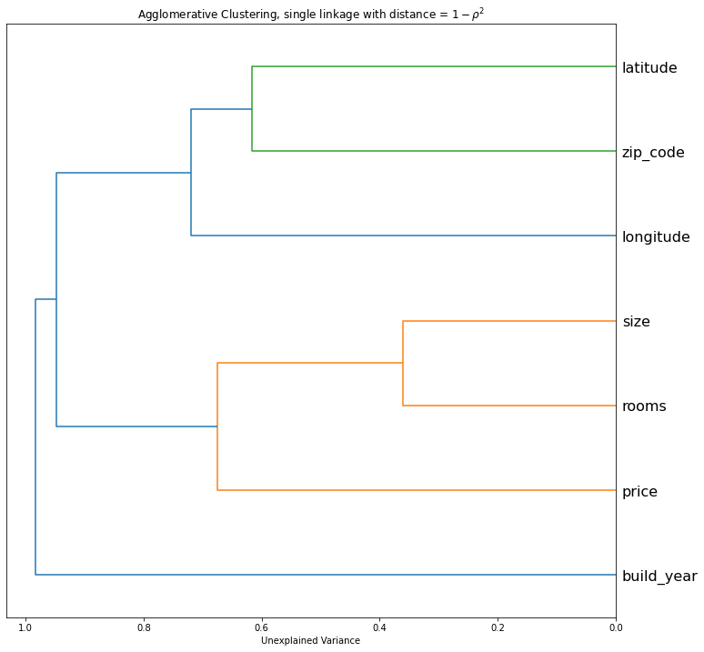

Correlation Clustering

References

Comments